
GPS provides 24/7 location information to you anywhere on the globe, or in near-Earth space. It's a wonderful utility that helps people around the world find their way and know the exact time. Because GPS uses satellites moving in a 12 hour orbit around the Earth, and because of other inherent errors in the GPS system, your location as provided by GPS varies in its accuracy. Much like the weather, GPS accuracy varies over the days, weeks and months.
We understand why GPS has errors, even if we can't completely eliminate them. Because we understand them, we can predict them with good success.
There are two things that contribute to GPS errors:
Because GPS satellites are in a Medium Earth Orbit (MEO, about 20,000 Km), they orbit the Earth twice in one day. The satellite's position above any given location will repeat with that frequency too. To get a 3-dimensional position fix from GPS, you need navigation signals from at least four GPS satellites. The fourth one is required to get the exact time, since the clock in your GPS device is not that accurate.
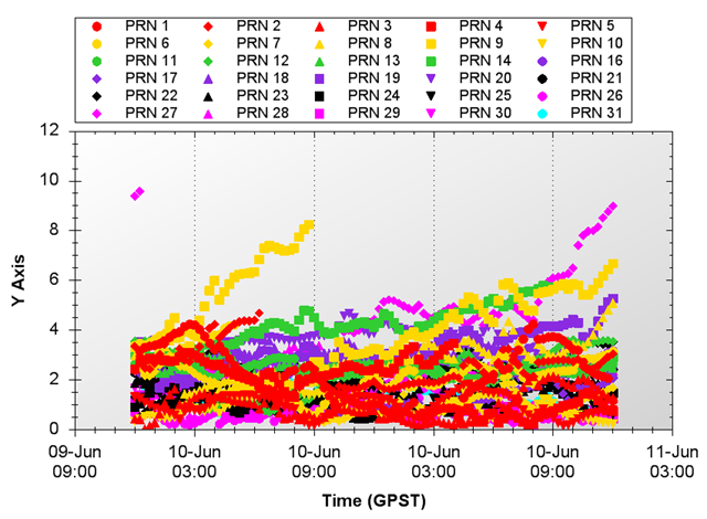
The same sets of GPS satellites will be overhead at roughly the same time twice a day, so you will have roughly the same accuracy at the same time each day. Technically, the same satellite orientation will occur, leading to the same accuracy, four minutes earlier each day. GPS orbits repeat twice in a SIDEREAL day, while we keep time on a SOLAR day. So, if Item 2 above was the same for all satellites, you'd get repeatable, predictable accuracy just by knowing the positions of GPS satellites. In the graph above, notice where the spikes and dips happen. These occur when GPS satellites either drop below the horizon (causing a spike) or come into view above the horizon (causing a dip). The more satellites you have in view, the smaller your positioning errors will be. Four is the minimum number your need, but the navigation equations allow for any number of navigation satellites to determine your position.
The GPS satellite's URE is also a factor in your accuracy. Your GPS device implements the navigation equations to determine its position, using information provided by each GPS satellite. The navigation equations require that the GPS satellite's position be known, and also the time the information is sent, as measured by the GPS satellite. Determining your location is done by calculating the distance from your location to the satellite (by measuring the time it took for the signal to travel from the satellite to your device), and then combining that with similar measurements to other satellites. Knowing the distance to each satellite, and the satellite's position, the navigation equations determine your position.
However, to achieve this each GPS satellite must track time very precisely, and be able to send down its precise location. Precise time is kept on each GPS satellite by an atomic clock. Each satellite has 3 or 4 of them, but only one is used at a time; the others are spares. Even though atomic clocks can keep time very accurately, they still produce unpredictable errors. When measuring distances using timing signals from satellites, an error of one nanosecond leads to about 1 foot of error. Most GPS satellites are accurate to about 5-10 nanoseconds.
A GPS satellite's position is determined by the satellite operators on the ground, and then sent up to each GPS satellite so that it can send that position information down to your device. Operator's the the Second Space Operations Squadron (2SOPS) predict GPS satellite orbit data for weeks in advance. Orbit predictions have errors in them though, so as the satellites send down their information, operators from 2SOPs check how well their predictions were, and upload new orbit data when necessary. GPS orbit data is usually accurate to 10-20 feet.
Both the GPS orbit data errors and the precise clock timing errors combine to make the URE. The URE is inherent in the navigation signal you receive at your device and adds to the location error you are experiencing at any given time. The good news is that these errors can be categorized statistically and plots like the one above can be used to understand your GPS location error.
There is a difference between predicting your accuracy, and assessing your accuracy with GPS. For the predictions, you're estimating the satellite position in the future as well as the satellite's clock behavior. If you want to know precisely what your GPS errors were in the past, you can use a different type of data and perform an accuracy assessment.
The articles on assessed and predicted navigation accuracy below were written when I was the author of The Nog, the Navigation Blog at AGI. They explain more in depth the differences between the two types of accuracy determination - in a way that only The Nog can.
Assessed navigation accuracy is a term I use to define a navigation accuracy calculation that uses actual navigation constellation error data. When an accuracy calculation is performed, many different types of data can be used. In this article, I'll focus on the errors inherent in the control and space segments of GPS.
One of the larger error sources in you position estimation (now that Selective Availability is turned off) are the errors induced by inaccuracies in the navigation satellite's ephemeris and clock states. These errors are uncorrectable by the user who does not have a differential system such as the USCG National DGPS system or the FAAs WAAS system. With a differential system, a base station or stations can observe the satellites in view and determine the ephemeris and clock errors. Once calculated, these base stations will communicate what these errors are to an appropriately equipped receiver. Details of how DGPS and WAAS work will be covered in a future article.
Navigation satellite ephemeris errors result as a difference from the satellite's broadcasted position and the its actual position. As part of the required data for a navigation solution, the navigation satellite broadcasts its position to your receiver. The receiver takes this position as truth and uses it in the navigation equations to calculate its position.
The navigation satellite gets its position data from the control segment, which it predicts typically for 24 hours in advance. These control segment predictions are very accurate at the time of prediction, but as time progresses (as the Age Of Data increases, as they say) the predictions are further and further off.
The same type of process results in the clock state for the satellite. Just as satellite orbit positions need to be predicted, so do atomic clock phases and frequencies. Satellite orbits are well understood, but there are still small, unmodeled perturbations which affect the orbit that predictions don't take into account. For atomic clocks the errors are induced by quantum behavior in the device itself. No amount of modeling can predict the clock state exactly; we typically rely on 2nd order fits of the clock state to make the predictions that are uploaded to the satellites.
So now we know where the constellation errors come from - how are they applied to a navigation accuracy assessment? Before the satellite ephemeris and clock errors can be used, they must first be determined - and that will be the topic of the next article.
As mentioned in the previous post, these errors are the same (mostly) as those broadcast by dgps systems - so how do dgps systems determine the errors? Its actually pretty cool. We know how a receiver works - it moves and its position updates as it moves around - the position being calculated by the governing navigation equations. Suppose the receiver was fixed at a known (surveyed) location? Its location is no longer an unknown in the navigation equations - now we can take the satellite position as an unknown and solve for it instead. Since the satellite is broadcasting its precise (predicted) position, we can difference the two and get the ephemeris error. Easy.
What about the clock error? Well, we'd need a 'surveyed' clock state to compare the satellite's clock state against. This is achieved at some monitoring stations (as these fixed stations are known) by using a local atomic clock to compare states against. Other techniques exist as well, such as syncing to the USNO time standard.
Two problems occur when calculating the difference in this manner:
Let's look at the second problem first. Measured data is noisy by definition. Many types of measurement errors can be included in any measurement. One common resolution to this problem is to use a filter to smooth the measurements. In the case of GPS measurements, a Kalman filter is commonly used in practice. The output of the filter is a smoothed measurement, providing a better estimate of the ephemeris or clock error. We'll use this result to solve the first problem.
The first problem arises out of the fact that the differences are good for that location only. As you start to move away from the surveyed location where the difference was calculated, it becomes less and less correct. This is because the differences were determined using specific line-of-sight paths through the atmosphere - the farther you move away from the station, the more the line-of-sight paths change. How can you overcome this spatial decorrelation?
In practice at the GPS Master Control Station, (and in other operational global differential networks) this is overcome by using the smoothed estimate for the clock and ephemeris error for any location on the globe. There is a chance that the estimated error will diverge from the observed error, but the more surveyed stations there are supplying observations, the smaller the chance. Judicious measurement weighting and Kalman filter tuning can also reduce that likelihood.
So what do these ephemeris and clock errors look like over time? Which one affects your receiver's accuracy more? Is there a plot?
Sure. Here are the errors for the entire constellation for a whole day:
Ephemeris Errors
Clock Errors
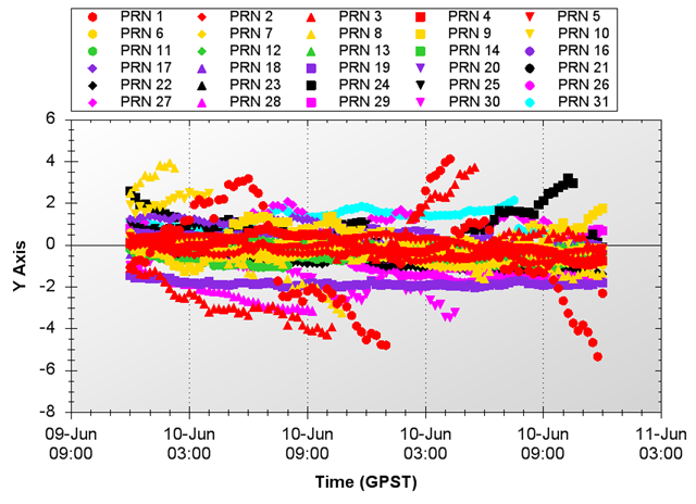
Notice how some of these errors tend to run off. This is the estimate diverging from the predicted, broadcast ephemeris or clock state. When these divergences get too big, new ephemeris predictions are made and a new upload is sent to the satellite, bringing the age of data back to zero and the ephemeris and clock errors back to zero (or close to zero). So how do these errors combine to provide the error your receiver will experience?
Ahhhh, now you have to wait until Part 3.
Ok, you've had some time to digest the first two parts of this series on assessed navigation accuracy. First I discussed what ephemeris and clock errors were, then I went over how those errors are created. Now, in this final installment, I'll show how these errors are are turned into accuracy measurements for your GPS receiver.
For now, let's assume that our only errors are those we've discussed - ephemeris and clock errors. There are other errors that affect your receiver and those are covered in the GPS Error Budget. See that section at the top of the page. Now that we know what our typical ranging errors are, we need to understand how those are translated into a positioning error.
The other piece of the error puzzle (and there are only two pieces) is Dilution of Precision (DOP). DOP is the effect that arises from measuring signals from spatially separated sources - be they lighthouses, GPS satellites, semaphore technicians or pulsars. DOP typically has the effect of diluting the accuracy of your ranging measurements. I'll cover DOP much more thoroughly in a future nog as well - because we want to get to the good stuff now!
Notionally, your receiver's accuracy can be modeled as:
receiver error ~ DOP x URE
This is not a mathematically robust description, but it does show the general behavior of your errors. The higher your DOP or URE, the higher your receiver's error. If you lower either, you're more likely to find that geocache quicker. The mathematically correct construct for DOP is a matrix, and the UREs are a vector. The elements of the URE vector are the total root sum square (RSS) errors along the line-of-sight from your receiver's antenna to each GPS satellite.
So far we've only discussed the ephemeris and clock errors, but any error can be RSS'd into the URE and be used in the receiver error calculation. You can see these other errors in the GPS error budget.
So, there it is, on the table - now you know how accurate your receiver's position estimates are. As long as you know all of the satellites ephemeris and clock errors at a given time (and all the other errors we glossed over) and you can do the matrix multiplications on the fly. Piece a cake! Right - we don't think so either. That's why we automated all the data collection and math for you in our tools.Here is a graph of the assessed receiver position error over a day, using just ephemeris and clock errors. So now, when you see or hear about assessed navigation accuracy, you know that means the actual errors from a time in the past were used to calculate the position errors.
Assessed Positioning Errors
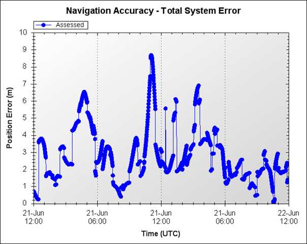
It's always nice to see where you've been, to see the wonderful position errors you had in the past - (like at 08:00 UTC in the graph!). But what good does that do you for tomorrow's buried treasure diving expedition? You need to be able to predict what these errors will be... and I will cover that topic - predicting GPS accuracy - in a future nog as well.
Navigation error prediction is an on-going science that so far has produced mixed results. The algorithms are generally the same for GPS accuracy prediction as they are for GPS accuracy assessments. If you have not read that section yet, I highly recommend it.
I should bound your expectations early, so you don't think that we can predict GPS errors a year in advance - typical prediction timelines for GPS errors work similarly to prediction timelines for the stock market and other volatile processes - the longer you want to predict for, the larger the error. For purposes of our discussion, we'll be looking at days and possibly weeks of GPS error prediction - nothing longer.
Since GPS navigation accuracy is a function of both dilution of precision (DOP) and each satellite's individual user range error (URE), we need to look at how well each can be predicted. DOP predictions were covered at length in this article I wrote for the December 2008 issue of InsideGNSS. It turns out that DOP can be predicted quite well for weeks into the future, especially if there are no intervening satellite outages. That being the case, I'll focus this article more towards predicting the URE portion of the navigation error.
Each GPS satellite broadcasts it's position in space along with other pertinent information to your GPS receiver. That position, combined with the timing information embedded in the signal itself, allows your receiver to calculate the distance to the satellite. The error in that distance calculation is called the user range error and stems from inaccuracies in the satellite position and clock information as well as errors introduced by ionospheric and tropospheric refractions.
The satellite and clock errors together combine to create what's termed the Signal-In-Space URE (SISURE), while the addition of the atmospheric errors and other positioning errors the receiver itself provides combine to create the commonly named User Equipment Range Error (UERE). In this post, I'll focus on the SISUREs, leaving the full URE for a further topic of investigation.
I've broken the navigation error prediction problem into constituent pieces, and am now focusing on a small (but feisty!) piece of the puzzle. Implicit in this process is the fact that I can recreate the full navigation error once I determine the predicted error in the URE. What the heck, let's assume that for now!
Because we're determining a range to the satellite, any errors we want to predict must lie along the line between the receiver and the satellite. By definition, timing, or clock errors are always along this line, but only the radial portion of the satellite position error lies on this line. Typically, the SISURE is determined by subtracting the satellite's radial position error from the satellite's clock error:
SISURE = Radial error - Clock error
What does the SISURE look like? The best way I know of to start predicting something is to look at it and see what patterns can be seen and possibly repeated. Here's a plot of the SISURE values for the entire GPS constellation of satellites on a given day:
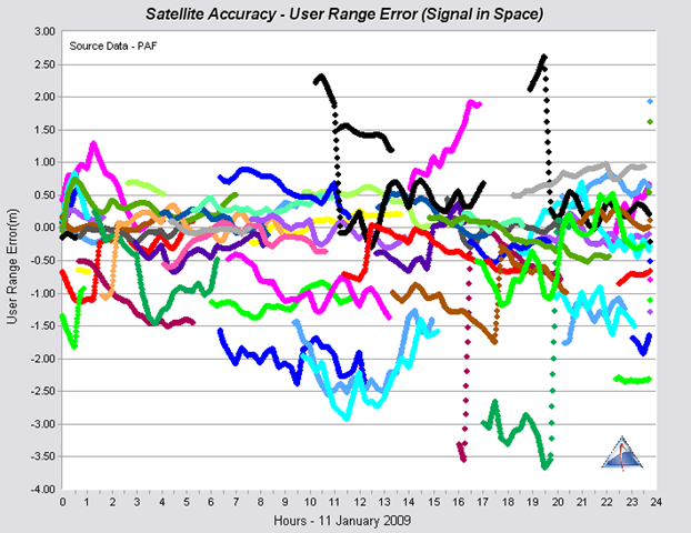
Ok, one look at this picture shows us that trying to fit some kind of periodic function to predict the behavior is not going to be easy. So what options are available? How could we use this data to predict future GPS behavior? I'll let you mull over that while you sip your Nog and continue with my thoughts on the subject in the next installment. Until then, good travels.
In the last section we left off trying to figure out how to predict GPS behavior from the data I showed you. Our GPS error prediction problem involves predicting the Signal-In-Space User Range Error (SISURE), to the extent possible. From Figure 1, we came to the conclusion that trying to fit some type of periodic function to this data was going to be difficult. So, where do we go from here? In situations like these, I'll always recommend that more data analysis can help, and this case is a perfect example.
Figure 1 above shows only one day's worth of SISURE values - the next question we should ask ourselves is, is their a long term behavior to this data? Let's find out.
gathered over 800 days of SISURE data, and looked at the maximum clock error, ephemeris error and the combined user range error for that period. The following plots show what the maximum errors look like. To keep the plots readable, I've only plotted two satellite's worth of data in each.
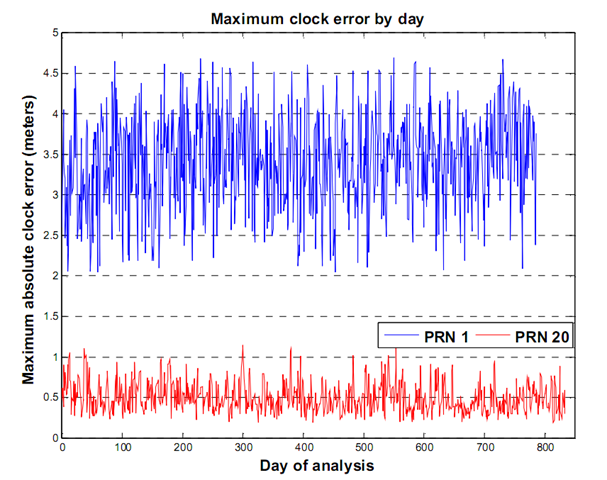
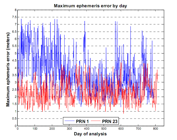
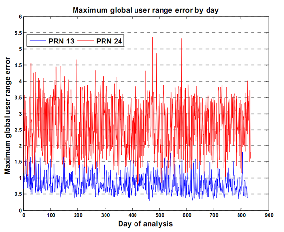
These plots show something good. The errors in both clock and ephemeris (and hence the SISURE) are clamped. This means that they do not grow past a certain value - a value we can estimate and use to our advantage. Even when the errors oscillate over the day, we can say that on average, the errors will not go above some value. This clamping behavior is not a result of GPS system mathematics or design stability. It's the direct result of active participation and monitoring by the United States Space Force 2
This may be old information to some, but I want to be clear on why these errors do not grow. The GPS system continually broadcasts its position and clock state information to users world wide. The information the satellites broadcast was predicted by 2SOPs and uploaded to the satellite roughly 24 hours earlier. When this predicted data is sent to a GPS satellite by 2SOPs it's called a nav upload. Nav uploads only occur when they are necessary, that is, when a satellite's predicted position differs from its actual position (that's the Kalman Filter's estimated position). So the maximum error a satellite will broadcast is determined by 2SOPs - they do the clamping. Without this clamping, we would see errors that increase roughly quadratically over time. Thanks 2SOPs!
Looking at the above graphs, we can see that using an average of the errors will give us a good number to use in our predictions. There are long term trending issues, especially with PRN 1's ephemeris error in this case, so we'll have to take our averages over shorter periods. These average values will help us predict our GPS accuracy statistically, over longer periods of time. Obviously, we can't use these numbers to predict the short term behavior of the SISUREs, but we can identify how each satellite performs and get statistical estimates of GPS accuracy for longer periods.
This is where Prediction Support Files (PSF) are used. If you've used AGI's Navigation ToolKit or the AGI Navigation Accuracy Library Component at all, you'll be familiar with PSF files. A PSF file contains the root mean square values (RMS) of the ephemeris components and the clock for each satellite over the last seven days. Graphs of all PSF files are available here, see the second graph on the page. Here's the graph from today:
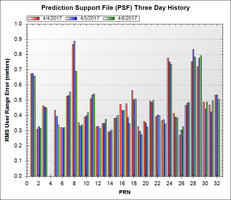
You can see that some satellites perform much better than others, and it's this type of differentiation we want to take into account when predicting GPS accuracy.
Warning: Statistics Ahead!
Using this PSF data, we can predict GPS accuracy. We cannot predict specific errors in a given direction (East, North, etc.) but we can predict a statistical GPS error for any location given a confidence level we want to use. In the assessed navigation accuracy section, I outlined how to generate GPS errors from a previous time using Performance Assessment File (PAF) data. Using that same method, we can use Prediction Support File (PSF) data to generate future GPS errors - but only the RMS value of the error - not the actual error. The RMS values produced from the GPS navigation accuracy algorithms have probability distributions associated with them, depending on the dimensionality of the prediction we are using.
One-dimensional predictions, like east error, vertical error or time error, will have the standard one-dimensional Gaussian probability distribution. This means that the RMS prediction of these values will have a 68% probability of likelihood, 1 sigma. Multi-dimensional statistics are required for predicted values of horizontal error and position error. For the two dimensional horizontal error, the predicted RMS value has a 39.4% likelihood 1 sigma. Three dimensional position errors have a 19.9% likelihood 1 sigma. These 1 sigma values are not constant for the different dimensions, making comparisons difficult. These predicted values can all be scaled to a specific 1 sigma level, or confidence level, using scaling factors derived from past GPS error data.
For example, to compare the East, Vertical and Position errors, we would use different scale factors to convert the predicted RMS values for each of those metrics to a single, 95% confidence level. Theoretical scale factors are listed on the internet, but the theoretical values don't accurately model the behavior of GPS. AGI's STK Components Navigation Accuracy Library provides a way to use scaling factors derived from empirical data, more accurately representing the GPS constellation behavior.
The graph below shows the empirically derived scale multipliers, using over 600 days worth of data.
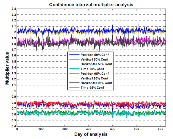
The tables below show the actual scale factors to use for the different metrics, with their associated errors.
50% Confidence Level Multipliers
| Dimensions | Empirical Value / Standard Deviation | Theoretical Value |
| 1 - Vertical | 0.6323 / 0.0223 | 0.6745 |
| 1 - Time | 0.6084 / 0.0220 | 0.6745 |
| 2 - Horizontal | 0.7824 / 0.0236 | 0.8326 |
| 3 - Position | 0.7551 / 0.0236 | 0.8880 |
95% Confidence Level Multipliers
| Dimensions | Empirical Value / Standard Deviation | Theoretical Value |
| 1 - Vertical | 2.0096 / 0.0316 | 1.960 |
| 1 - Time | 2.0230 / 0.0281 | 1.960 |
| 2 - Horizontal | 1.8109 / 0.0431 | 1.731 |
| 3 - Position | 1.8433 / 0.0380 | 1.614 |
So, using this scale data and the PSF data, what do my predictions look like? The graph below has the actual error in red. The 95% confidence predicted GPS accuracy is in blue and the 50% confidence predicted GPS accuracy is in green. Notice that roughly only 5% of the actual errors are above the blue line, and roughly 50% of the actual errors are above the green line. Notice also that the shape of the 50% line and the 95% line are identical. This is because they are the same prediction - just scaled differently.
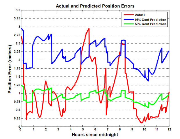
There's one more thing you should be aware of when predicting navigation accuracy. The confidence levels you pick won't always be adhered to. Because of the day-to-day variability of the GPS system, the multiplier values are not constant for a given confidence level. This is evident from Figure 6 above. In the Figure 7, the true percentage of actual errors above the 95% prediction line is 6.8%, not 5%. This makes me wonder, how long can I use a PSF file to predict my GPS accuracy before the PSF data, or the multipliers become too old to use?
To see if I could find out, I plotted the excursions (the percent of actual GPS errors greater than the predicted GPS errors) for 155 days, using the same PSF file. The PSF is brand new for day 1, but as we head towards day 155, the PSF file becomes increasingly older. If there is any correlation between older PSF data and GPS accuracy prediction, we'll be able to see it.

The graph says it all - there is no difference in the number of excursions based on PSF age. If there were, we'd see an increasing trend from left to right, meaning more actual errors were breaking the 95% confidence threshold. This implies that a PSF file is good to use for longer periods of time, but in using one, you must expect that sometimes the GPS errors will be worse that you expected.
If you've made it this far, congratulations! The topic is not an easy one and you have to be a die-hard stats fan to keep at it. Enjoy your Nog and tell everyone at your next party that you know GPS prediction excursions aren't constant, but can they tell you why?
Next time, I'll cover the art of short-term GPS error prediction. We'll move away from stats for awhile, but we may ask Taylor for a little help... Until then, smooth sailing.
In Part 2, I wrote a Nog on predicting GPS navigation errors in the long-term - over days and weeks. In this Nog, I'll cover predicting short term navigation errors, which is a little more tricky believe it or not. This is because for long-term errors, we can use statistics to predict the general behavior of GPS clocks and ephemeris, distilling that down into a statistical position error prediction. That type of prediction results in an error covariance, an error ellipsoid around the true position. For the short term (several hours), we have access to the latest clock and ephemeris errors and by using them we can create a predicted error vector, which is a better thing to have.
The difference between an error ellipsoid and an error vector can be explained by example. Suppose you lose your car keys. Having an error ellipsoid may tell you that they are in your house somewhere, which is not too bad of a search but you have to search the entire house. If you have an error vector, it would tell you that they are under last weeks mail near the kitchen junk drawer - much better information! A lot less searching.In the navigation world, and error ellipsoid tells you the treasure is in the general area, but an error vector points to the giant X on the map.
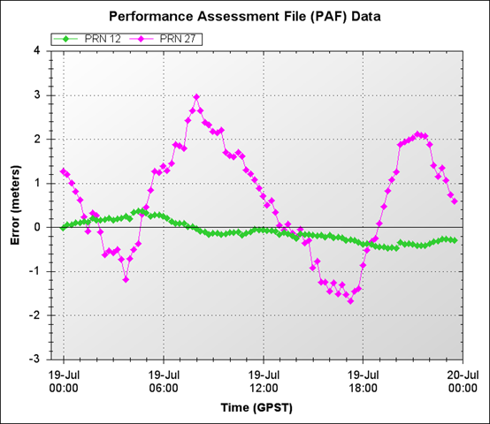
So, now that we have a basic understanding of the types of errors, let's look at how we might use the data we already have (in a PAF file) to predict error vectors for several hours. If you're not sure how a PAF file leads to a navigation error assessment, be sure to catch up by reading the Assessed Errors section. An initial thought would lead us to perform a linear extrapolation of the the data in a PAF file. This will definitely produce navigation accuracy predictions, but not ones you'd want to use to search for your keys. The plot below shows how the navigation error prediction grows dramatically as time goes on. This is just not good at all, in fact, I'd call this prediction: FAIL. In the plot, the data prior to 12:00 is actual data, the data after 12:00 is predicted, based on the data before 12:00. The linear extrapolation routine uses the information in the last data points of a PAF file, and extrapolates them based on their value and the values rate of change (first derivative).

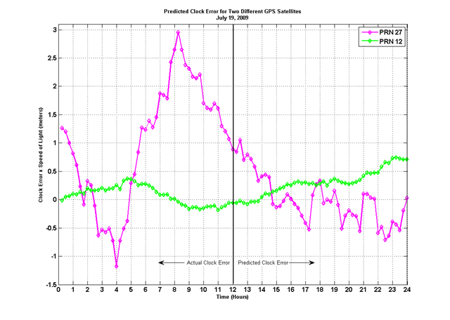
So, besides linear extrapolation what else can we do? I spent a lot of time thinking about this and I've come up with an algorithm that better mimics the PAF data and leads to much better predictions. There are further refinements I can make to this algorithm, but I wanted to share the results I have so far. The plot below shows two different satellite's clock errors - a major contributor to the navigation position error. This plot was taken directly from the GPS Satellite Performance page here.
With such different behaviors amongst satellites, I needed a method of prediction that was also varied. The first cut at the prediction algorithm produced the results below:
These results are in the ballpark! We're now getting closer to our navigation error prediction. Using the same prediction algorithm on all data in the PAF file, using the same scheme as before, data before 12:00 is actual, data afterwards is predicted, I generated 30 samples of predicted PAF data. The prediction algorithm is based on random numbers, so 30 different samples will all look different. With these samples, I plotted them with the truth navigation error to see how well we faired. This plot shows the results:
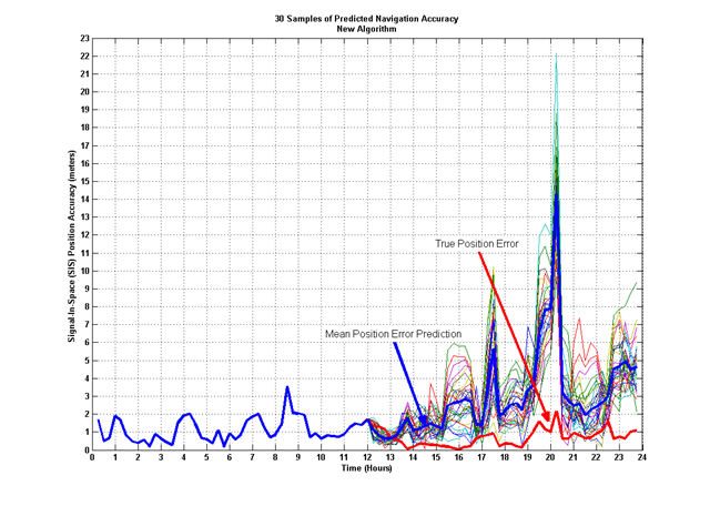
The thick red line shows the true position error, and the thick blue line shows the mean of the 30 prediction samples. The other lines each represent one of the 30 predictions of the navigation position error. These results are much better than the linear extrapolation method from above. We can see the effect of Dilution of Precision (DOP) on the accuracy - where the truth data rises, we see similar rises in the predicted accuracy, but because half of the navigation accuracy calculation is based on data that is inherently random, we'll never match exactly. The idea here is to get as close as we can. I'd much rather use this new algorithm to find my lost keys - at least I know they are still somewhere near the kitchen!
Prediction is a tricky game, but the better we understand the problem, the more likely we are to get a better prediction. I'll keep working on improvements to this algorithm, in the mean time, let me know your thoughts!. My brain hurts, it's time for a Nog.
Smooth seas...
The GPS error budget contains the errors that typically exist when your GPS receiver makes a ranging measurement to a GPS satellite. Some of these errors can be corrected by your receiver, others cannot. The values list in an error budget are those that remain after your receiver corrects what it can.
Different error sources are usually binned into different categories, such as Signal-In-Space (SIS), Atmosphere or Receiver. Here's a typical error budget for GPS:
| Error Type | Error (meters) | Segment |
| Ephemeris | 3.0 | Signal-In-Space (SIS) |
| Clock | 3.0 | Signal-In-Space |
| Ionosphere | 4.0 | Atmosphere |
| Troposphere | 0.7 | Atmosphere |
| Multipath | 1.4 | Receiver |
| Receiver Noise | 0.8 | Receiver |
| Total (URE) | 6.09 |
These errors are one-sigma values. The total is arrived at by root-sum-squaring (RSS) the individual errors.
All of these error sources are dynamic and modeling is harder for some, easier for others. The SIS and atmosphere errors are along the line-of-sight from the receiver's antenna to the GPS satellite.
This is one GPS error budget, other error budgets exist as well.
You can determine your GPS accuracy at my new site: https://gpsoutage.com/gpsaccuracy
Gps Basics
The basics of how GPS works with some technical content.
How Long Can You Use an Almanac?
GPS position data is contained in almanac files. Learn how long you can use these for analysis.
Quantitative Analytics for BVLOS Operational Risk Assessments
Using quantitative analytics, we show that functions describing metrics of interest in BVLOS ORAs can be used to define risk likelihood. This leads to a way to automate operational risk assessments, and visually display risk likelihood for faster, more accurate UAV operator decision making.
Understanding GPS Navigation in Contested Environments
Review of GPS errors, their source and how we can mitigate them. Review of terrain datums and their operational usage and an overview of alternative navigation techniques.
Operational Considerations for Improved Accuracy with an IOC Galileo Constellation
This paper looks at how the Galileo operators can improve the performance of an initial Galileo constellation by managing their ephemeris and clock errors. Keeping those errors small can help keep initial positioning errors small, even when large DOPs are present.
Long term prediction of GPS accuracy - Understanding the Fundamentals
Topics on prediction methods for GPS and how long GPS errors can be predicted. Starting from an understanding of the elements of prediction, including almanac use and ephemeris and clock errors, I look at the statistics of GPS position error predictions under various scenarios.
Statistical Analysis of Military and Civilian Navigation Error Data Services
This paper examines the difference between ephemeris and clock errors generated using civilian data versus those generated using military data. The different data sources result from civilian GPS receiver and military GPS receiver.